Bonding Curve in Crypto Explained: How Token Price & Supply Connect

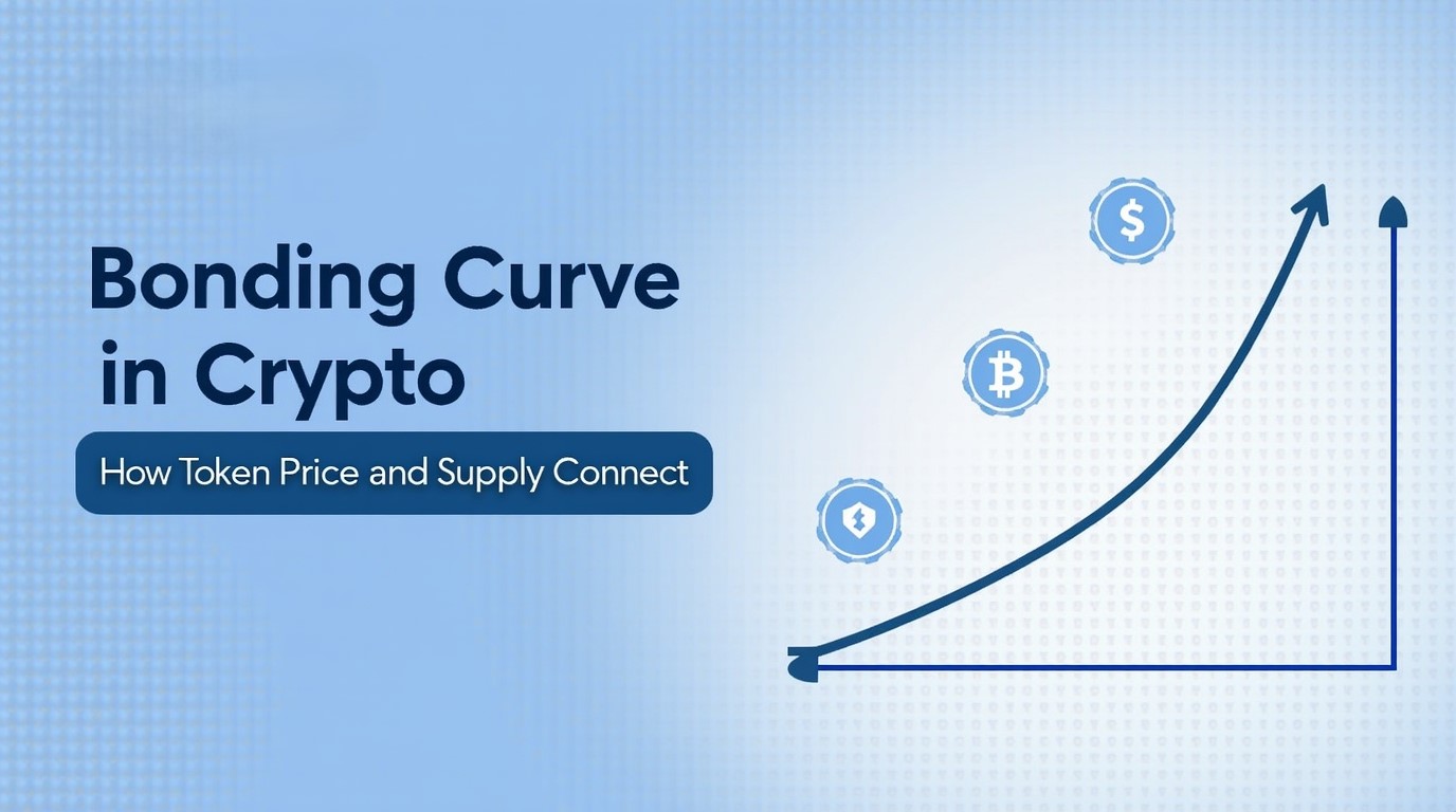
Picture a concert where every ticket sold makes the next one slightly more expensive. The earlier you buy, the cheaper it is, but as demand grows, prices climb automatically. That is the essence of a bonding curve: a simple yet powerful idea that automatically links a token’s price to its supply. Instead of relying on buyers and sellers to negotiate in an order book, bonding curves use mathematical functions built into smart contracts to set prices in real time.

Why does this matter? Because in crypto, predictable and transparent pricing is the difference between chaotic speculation and sustainable growth. Bonding curves ensure continuous liquidity, reward early adopters, and give projects a fair, automated way to launch tokens without centralized exchanges.

This blog will walk you through the basics of bonding curves, show how different curve shapes affect token pricing, and explain why they are becoming a cornerstone of Web3 tokenomics. Whether you are new to crypto or curious about dynamic pricing models, you will see how bonding curves connect supply and demand in a way that is both elegant and beginner-friendly.

What is a Bonding Curve?

A bonding curve is a mathematical rule that automatically sets a token’s price based on how many tokens exist. As more tokens are bought, the price rises along the curve; as tokens are sold, the price falls. This makes token markets predictable, liquid, and fair without the need for traditional exchanges.

A bonding curve is a graph that shows the relationship between token supply (x-axis) and token price (y-axis). It is powered by a smart contract that enforces the rule:

• Buy more tokens → supply increases → price goes up. 
• Sell tokens → supply decreases → price goes down.

Think of it like a vending machine, where each soda costs slightly more than the last one. A mathematical function defines the bonding curve:

                                                                   P = f(S)

where P = price and S = supply.

For example, if the curve is exponential, the price rises quickly as supply grows. If it is linear, the price rises steadily. Early buyers receive lower-priced tokens, whereas later buyers pay more because supply has increased. Bonding curve matters in crypto because;

• Liquidity without exchanges: Bonding curves embed liquidity directly into the token’s smart contract, so you don’t need order books or market makers.
• Fair pricing: Everyone knows how the price will change as supply grows, with no hidden manipulation.
• Incentives for early adopters: Early participants benefit from lower prices, encouraging community growth.
• Programmable markets: Projects can design curves to match their goals, with slow, fast, or capped supply.

Bonding curves are like automatic pricing machines for tokens. They ensure there is always a way to buy or sell, that prices are predictable, and that communities can grow without relying on big exchanges.

Different Types of Bonding Curve in Crypto Models

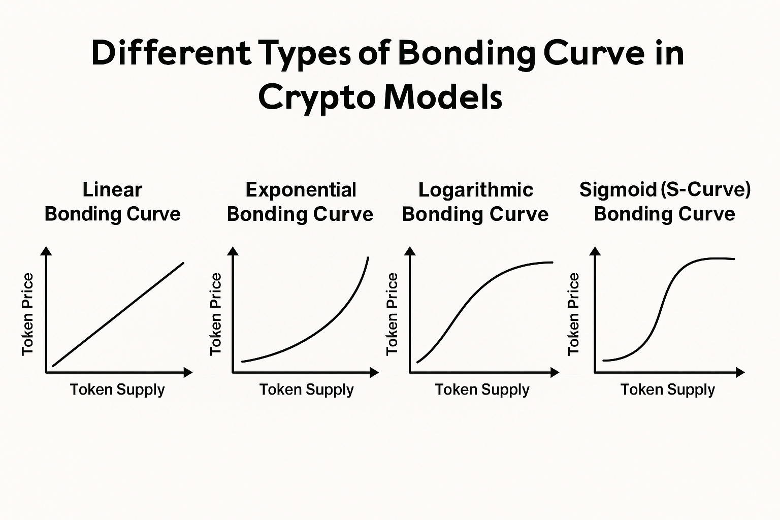
Bonding curves are not one-size-fits-all. In crypto ecosystems, different mathematical shapes can be used to define how token prices evolve as supply grows. Each curve creates unique pricing behaviors, incentives, and community dynamics. Choosing the appropriate bonding curve is crucial because it directly affects tokenomics, including token distribution, early-adopter rewards, and sustainable growth. Projects may select a curve based on their goals: steady transparency, strong scarcity, affordable late entry, or balanced adoption. Let’s explore the main types of bonding curves and why they matter.

Linear Bonding Curve

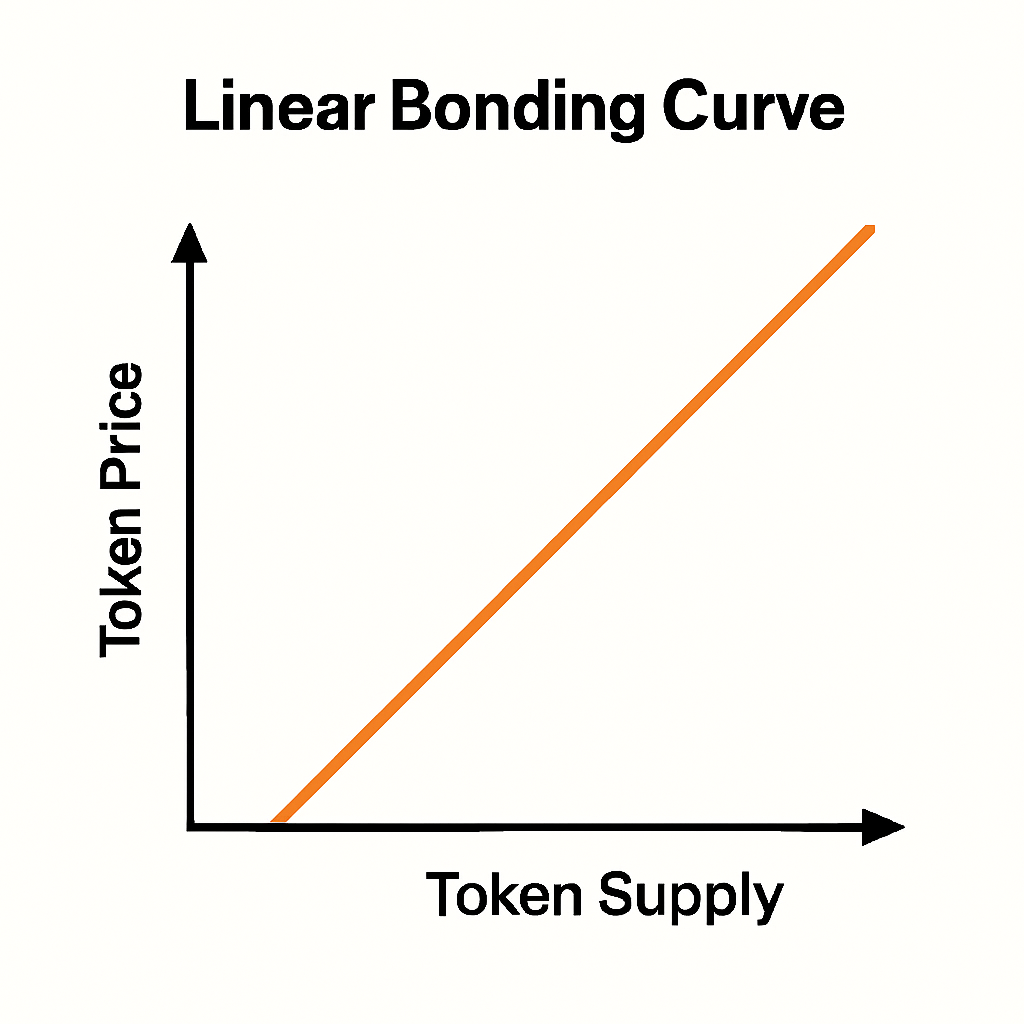
A linear bonding curve increases token price at a steady, predictable rate as supply grows. Imagine a straight line: every new token minted costs slightly more than the last, but the increase is consistent. This model is often used when projects want simplicity and transparency. It ensures that participants can easily understand how prices will change, making it beginner-friendly and fair.

Linear curves are well-suited for community-driven projects, educational tokens, or systems where predictability is more important than complex incentives. They discourage speculation by preventing sudden price jumps, and they provide a clear roadmap for token growth. By keeping things straightforward, linear bonding curves build trust and reduce confusion in token ecosystems.

Exponential Bonding Curve

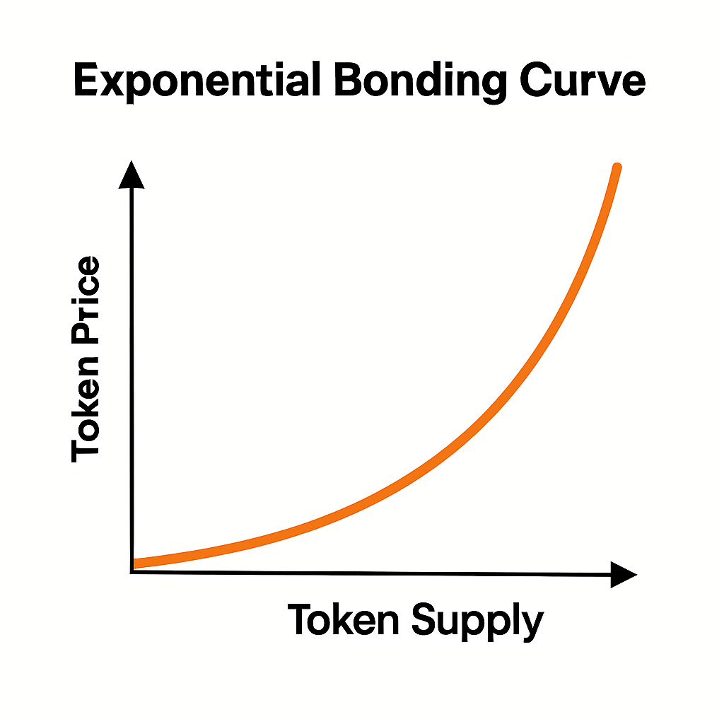
An exponential bonding curve starts gently but rises sharply as supply increases. Early tokens are inexpensive, but as more are minted, the price increases rapidly. This model is effective for projects that aim to emphasize scarcity and provide strong incentives for early adopters. It creates a sense of urgency for early adopters who benefit from low prices, while later participants face rapidly rising costs.

Exponential curves are often used in projects where demand is expected to grow quickly, or where exclusivity is part of the value proposition. They can also be applied in fundraising models that reward early supporters for taking risks. However, exponential curves can create steep barriers for latecomers, so they are most effective in ecosystems where scarcity is intentional and high-value participation is the goal.

Logarithmic Bonding Curve

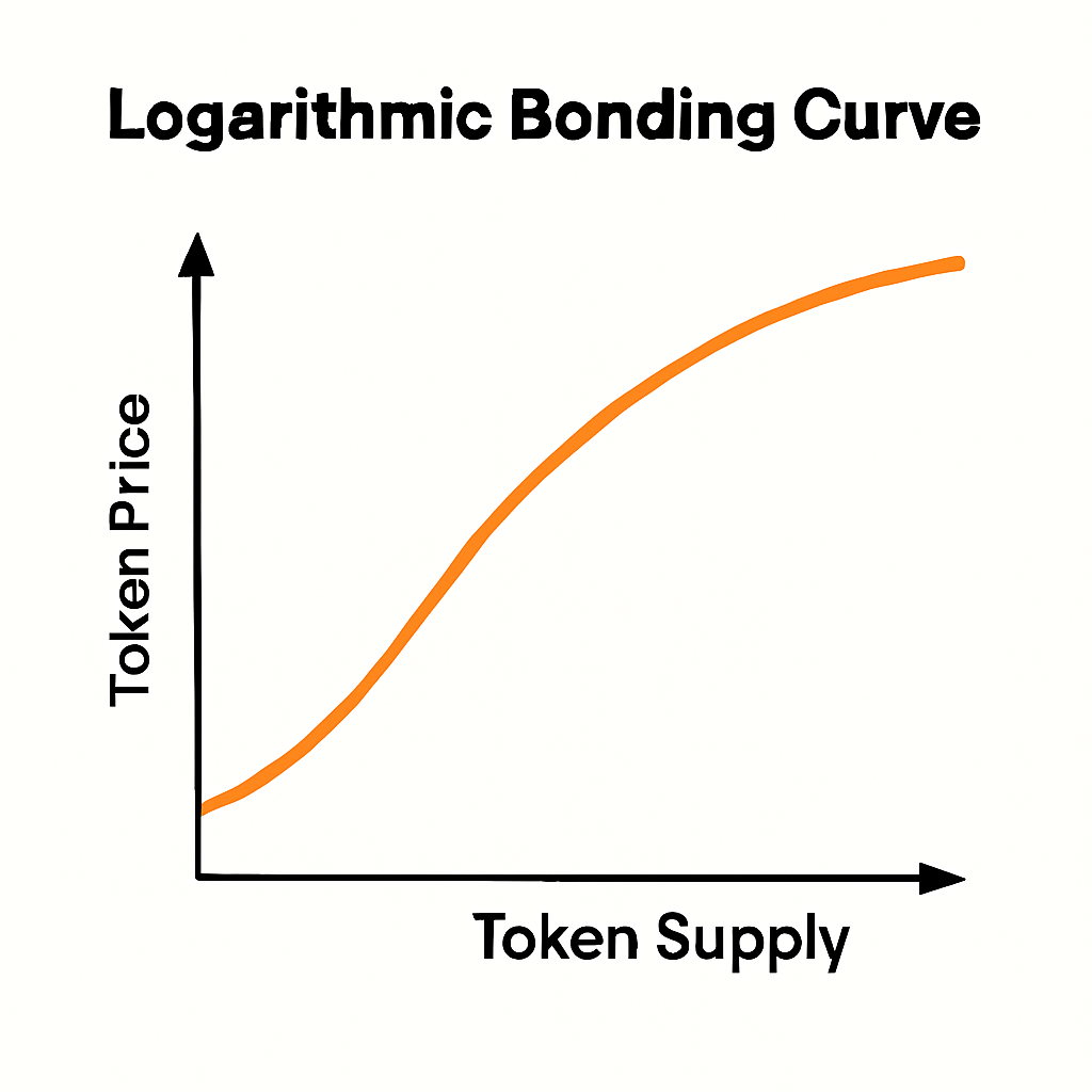
A logarithmic bonding curve rises quickly at first, then slows down as supply grows. This means early adopters enjoy significant rewards, but later participants can still join at affordable prices. The curve starts steep, encouraging early community growth, but flattens out to prevent runaway costs.

Projects use logarithmic curves to balance early incentives with long-term accessibility. It is a means of rewarding pioneers without penalizing latecomers. This model is particularly useful for community tokens, social projects, or ecosystems where inclusivity is important. By slowing price growth over time, logarithmic curves help maintain sustainable adoption and reduce the risk of speculative bubbles. They strike a balance between rewarding risk-takers and keeping the door open to broader participation.

Sigmoid (S-Curve) Bonding Curve

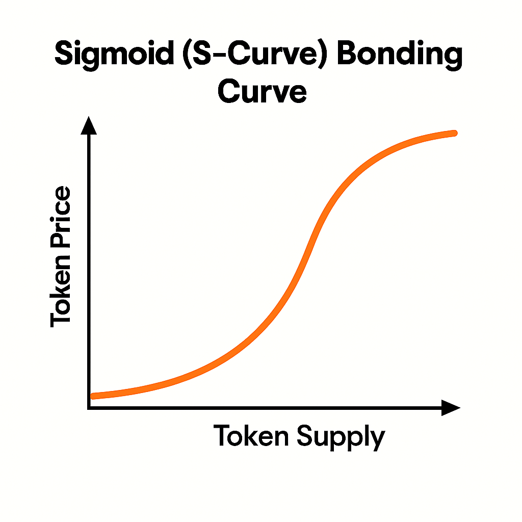
A sigmoid bonding curve, also known as an S-curve, grows slowly at first, accelerates in the middle, and then flattens out again. This shape supports balanced adoption by reducing speculation in the early stages and preventing late-entry barriers. Early participants don’t face extreme price jumps, while mid-stage growth creates momentum and excitement. As the curve flattens, it stabilizes the ecosystem, preventing prices from spiraling out of control.

Sigmoid curves are often chosen by projects that want to encourage steady, organic growth and discourage pump-and-dump behavior. They are ideal for community-driven ecosystems, DAOs, or platforms where long-term sustainability is more important than short-term hype. By smoothing out both ends of the curve, sigmoid bonding models achieve fairness across different adoption phases, making them among the most balanced approaches in tokenomics.

Bonding Curves vs. Traditional Market Pricing Models

Bonding curves use mathematical models to automate token pricing and liquidity, whereas traditional markets rely on human buyers and sellers to set prices through supply and demand. Bonding curves provide continuous, predictable pricing, whereas traditional order books offer dynamic but often fragmented price discovery.

Feature	Bonding Curves	Traditional Order Books
Pricing Mechanism	Algorithmic (based on supply)	Market-driven (bids and asks)
Liquidity Source	Smart contract reserve	Buyers and sellers
Price Discovery	Deterministic and continuous	Dynamic and emergent
Execution	Instant via smart contract	Depends on matching orders
Slippage Risk	Minimal (predictable curve)	High during volatility or low volume
Transparency	Fully visible pricing formula	Opaque until orders are placed
Use Cases	DAOs, NFTs, fundraising, DeFi protocols	CEXs, traditional assets, high-volume tokens

Bonding curves are smart contracts that use mathematical formulas to set token prices based on supply. As tokens are minted or burned, the price curve automatically adjusts. This creates continuous liquidity, as you can always buy or sell at a known price. There’s no need for a counterparty or waiting for someone to match your order.

• Price = f(supply): The curve defines how price changes with each token bought or sold.
• Liquidity is built in: The contract maintains a reserve (typically ETH or stablecoins) to facilitate trading.
• No order book needed: You interact directly with the curve, not other traders.

This model is well-suited to low-volume assets, NFTs, DAOs, and DeFi fundraising, where traditional liquidity may be thin or unreliable.

Order book markets (used by centralized exchanges like Binance or Coinbase) rely on buyers and sellers placing orders. Prices are determined through bid-ask matching, with the highest price someone is willing to pay meets the lowest price someone is willing to sell at.

• Liquidity depends on users: No buyers = no sales.
• Price discovery is dynamic: Driven by market sentiment, news, and speculation.
• Execution may be delayed: orders may remain unfilled or experience slippage.

Order books are better for high-volume assets, real-time trading, and speculative markets, but they can be fragmented, volatile, and opaque.

Benefits of Using Bonding Curves in Crypto Projects

Bonding curves are more than just pricing tools. They are foundational mechanisms that shape how tokens are bought, sold, and valued over time. Here’s how their core benefits support healthier token ecosystems:

• Transparent Pricing: Prices are set by a publicly available formula, typically based on supply. Everyone can see how the price will change as tokens are minted or burned. This eliminates hidden fees, manipulation, or opaque order books. Projects build trust with users by offering predictable, fair pricing from day one. Early adopters know what they’re getting into, and sudden price spikes don’t catch latecomers off guard.
• Continuous Liquidity: Bonding curves embed liquidity directly into the smart contract. Users can buy or sell tokens at any time, without a counterparty or an exchange—the contract reserves (e.g., ETH or stablecoins) to facilitate trades. Projects don’t need to bootstrap liquidity or attract market makers. This makes it easier to launch tokens and maintain healthy trading activity even with low volume.
• Fair Distribution: Early buyers pay less, and later buyers pay more, depending on the curve’s shape. Projects can design curves to reward early adopters, discourage whales, or cap supply. There are no pre-mines or insider deals, as everyone faces the same pricing logic. Token launches become more inclusive and merit-based. Communities grow organically, and speculation is reduced through thoughtful curve design.
• Automation via Smart Contracts: Bonding curves are fully automated, with no manual pricing and centralized control. The smart contract handles minting, burning, pricing, and reserve management. This reduces overhead, human error, and governance complexity. Projects scale more efficiently and stay decentralized. Teams can focus on building utility and community rather than manually managing token economics.

Bonding curves are especially useful for:

• DAOs: Transparent governance and fair member onboarding.
• NFTs: Dynamic pricing for limited-edition drops.
• DeFi: Automated market-making and fundraising.
• Social tokens: Rewarding early community support.

They help crypto projects launch faster, scale more effectively, and remain resilient; all while keeping users informed and empowered.

Common Challenges and Criticisms of Bonding Curve Models

Bonding curves, while powerful for automated token pricing, face several challenges: they can be complex for users, are vulnerable to manipulation and MEV (miner-extractable value) attacks, and are prone to slippage and volatility. These risks explain why some projects avoid them or use them cautiously.

• Complexity for Users: Bonding curves employ mathematical functions to determine price as a function of supply. For beginners, this can feel confusing and opaque compared with traditional order-book markets. Users may struggle to understand why prices rise or fall, especially when the price function is nonlinear (e.g., exponential, logarithmic, or sigmoidal). Lack of clarity can discourage adoption, as users prefer simple, intuitive pricing models.
• Potential Price Manipulation: Although bonding curves aim to reduce manipulation, vulnerabilities in smart contracts or poorly designed curves can still be exploited. Developers must ensure contracts are secure and resistant to attacks. If reserves are mismanaged, projects risk artificially inflating or deflating token prices. Trust in the project can erode if users suspect unfair pricing or insider advantages.
• MEV (Miner/Maximal Extractable Value) Risks: Bonding curve transactions are executed on-chain, meaning they are visible before confirmation. Bots or miners can front-run trades by inserting their own transactions to profit from predictable price movements. This creates unfair advantages for sophisticated players and disadvantages for regular users. Projects may lose credibility if users consistently face front-running losses.
• Slippage & Volatility: Large trades can cause significant slippage because each purchase or sale moves the price along the curve. In thinly traded projects, this can lead to extreme volatility, making tokens unattractive for everyday use. Unlike order books, bonding curves don’t allow partial fills or negotiation, as every trade impacts the curve directly. Traders may avoid bonding curve tokens if they fear unpredictable losses.

Some crypto projects avoid bonding curves because they introduce complexity that can be difficult for non-technical users to understand, thereby making adoption more difficult. While bonding curves promise transparency and automation, they also carry risks, including smart contract vulnerabilities, front-running or MEV attacks, and unpredictable slippage during large trades. If reserves are not managed properly, liquidity can collapse, leaving participants exposed.

Additionally, many users are more familiar with and comfortable with traditional order-book markets, where pricing feels more intuitive and less abstract. For these reasons, some teams prefer simpler, well-established models to bonding curves, especially when user education, security, and liquidity stability are top priorities.

As a creator, you should look out for the following pitfalls with the bonding curves;

• Overly complex curve design: Keep it simple and transparent.
• Smart contract vulnerabilities: Conduct thorough audits to prevent exploits.
• Reserve mismanagement: Ensure adequate collateral to back liquidity.
• Ignoring MEV risks: Consider protective mechanisms like batch auctions or private transaction relays.
• Poor communication: Educate users clearly about how the curve works.

Bonding curves can unlock powerful tokenomics, but they are not a silver bullet. Projects must balance innovation with usability, security, and fairness. Without careful design and education, bonding curves risk alienating users or exposing them to hidden dangers.

The Future of Bonding Curves in Web3 and Tokenized Economies

Bonding curves are still relatively new, but they are poised to play a major role in shaping the evolution of tokenized economies in Web3. As projects experiment with adaptive pricing, dynamic NFTs, and cross-chain liquidity, bonding curves are becoming more sophisticated, flexible, and integrated into next-generation token models.

1. Adaptive Pricing Models

Future bonding curves may become adaptive, meaning they can adjust their shape in response to market conditions, community activity, or governance decisions. Instead of being locked into linear or exponential formulas, projects could use dynamic curves that flatten during periods of volatility or steepen when demand surges. This would make token economies more resilient, balancing speculation with stability.

2. Dynamic NFTs

Bonding curves are increasingly being applied to NFT ecosystems, where each mint or burn event changes the price of the next NFT. In the future, dynamic NFTs could use bonding curves to reflect rarity, utility, or community engagement. For example, an NFT collection might start cheap, rise in price as demand grows, and then stabilize to encourage long-term holders. This creates programmable scarcity and fairer distribution without relying on hype-driven auctions.

3. Cross-Chain Liquidity

As Web3 expands across multiple blockchains, bonding curves could evolve into cross-chain liquidity bridges. Smart contracts may enable tokens to be bought or sold seamlessly across Ethereum, Solana, and other ecosystems, with bonding curves ensuring consistent pricing. This would reduce fragmentation and make token economies more accessible globally.

4. Smarter Token Issuance

Bonding curves can also enable more effective fundraising and token launches. Instead of fixed presales or centralized allocations, projects could use bonding curves to automatically issue tokens in response to demand. Early supporters benefit from lower prices, whereas later participants retain access to liquidity. This model could replace traditional ICOs with continuous, fair, and transparent token issuance.

5. Emerging Innovations

Emerging innovations in bonding curves are pushing the boundaries of how token economies can function in Web3. Projects are experimenting with governance-driven curves, in which DAOs can vote to reshape pricing models over time, thereby making tokenomics more democratic and adaptable. Others are exploring hybrid systems that combine bonding curves with automated market makers (AMMs), such as Uniswap, to create deeper liquidity and a smoother trading experience.

There is also growing interest in utility-linked curves, in which token prices adjust dynamically based on real-world usage, such as staking, voting, or in-game mechanics. Together, these innovations point toward a future where bonding curves are not static formulas but flexible, programmable economic engines that evolve alongside community needs and market conditions.

Final Thoughts

Bonding curves are more than just mathematical formulas. They are powerful tools for shaping token economies in Web3. By embedding transparent pricing, continuous liquidity, fair distribution, and automation directly into smart contracts, projects can launch with confidence, scale sustainably, and maintain healthier ecosystems without relying on centralized exchanges or market makers.

They make the most sense for projects that value predictability, inclusivity, and decentralization; whether it is DAOs onboarding members, NFT collections managing scarcity, or DeFi protocols designing innovative fundraising models. While bonding curves aren’t perfect and require careful design to avoid pitfalls, they represent a forward-looking approach to token issuance and community growth.

If you are curious about how bonding curves and other crypto innovations are shaping the future, join Dypto Crypto right now. We are a community built for real insights, fair reviews, and global perspectives. It is the ideal place to deepen your understanding and stay ahead in the ever-evolving Web3 landscape.

Frequently Asked Questions

Are bonding curves the same as AMMs like Uniswap?

No, bonding curves are not the same as AMMs like Uniswap. Bonding curves use a mathematical formula tied to token supply to set prices automatically, while AMMs rely on liquidity pools and constant product formulas to determine prices through trades. Bonding curves guarantee continuous pricing from a reserve, whereas AMMs depend on buyers and sellers interacting with a pool of assets.

Do bonding curves guarantee liquidity?

Bonding curves provide continuous liquidity because the smart contract always holds a reserve to buy or sell tokens. However, they don’t guarantee infinite liquidity, as liquidity depends on the amount of collateral locked in the reserve. Small reserves can lead to slippage or volatility, so proper design and funding are essential for stability.

Can bonding curves cause price manipulation or pump-and-dumps?

Bonding curves themselves are designed to reduce manipulation by using transparent formulas, but they are not immune to risks. Poorly designed curves, low reserves, or smart contract vulnerabilities can make them exploitable. On-chain visibility also exposes trades to MEV front-running, which can mimic pump-and-dump behavior. Careful design and audits are essential to prevent these issues.

Are bonding curves suitable for all token launches?

Bonding curves are not suitable for all token launches. They work best for projects that value transparency, automated liquidity, and fair distribution, such as DAOs, NFTs, or community tokens. However, for high-volume assets or markets that require complex trading features, traditional models such as order books or AMMs may be more effective.

What determines the “shape” of a bonding curve?

The “shape” of a bonding curve is determined by the mathematical function chosen to link token price with supply. Linear functions create steady increases, exponential functions rise sharply, logarithmic functions flatten over time, and sigmoid functions balance growth with stability.